Jupyter Notebook , Installation, Creating a Notebook , Detail

 What is Jupyter Notebook?

In this case, "notebook" or "notebook documents" denote documents that contain both code and rich text elements, such as figures, links, equations, ... Because of the mix of code and text elements, these documents are the ideal place to bring together an analysis description, and its results, as well as, they can be executed perform the data analysis in real time.

Launching the Jupyter Notebook

To run the Jupyter Notebook, open an OS terminal, go to ~/minibook/ (or into the directory where you’ve downloaded the book’s notebooks), and type jupyter notebook. This will start the Jupyter server and open a new window in your browser (if that’s not the case, go to the following URL: http://localhost:8888). Here is a screenshot of Jupyter’s entry point, the Notebook dashboard:

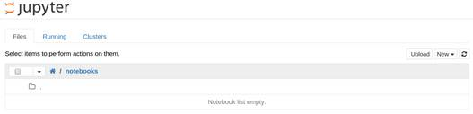
The Notebook dashboard

[box type=”note” align=”alignleft” class=”” width=””]At the time of writing, the following browsers are officially supported: Chrome 13 and greater; Safari 5 and greater; and Firefox 6 or greater. Other browsers may work also. Your mileage may vary.[/box]

The Notebook is most convenient when you start a complex analysis project that will involve a substantial amount of interactive experimentation with your code. Other common use-cases include keeping track of your interactive session (like a lab notebook), or writing technical documents that involve code, equations, and figures.

In the rest of this section, we will focus on the Notebook interface.

[box type=”note” align=”alignleft” class=”” width=””]Closing the Notebook server
To close the Notebook server, go to the OS terminal where you launched the server from, and press Ctrl + C. You may need to confirm with y.[/box]

Jupyter Notebook

Jupyter Notebook  is basically a web application. Unlike   IDEs (Integrated Development Environment), it uses the internet to run. And even after not being able to perform offline, it is highly preferred by most of the beginners because of its rich formatting and user-friendly interface. It allows us to enter the code in the browser and automatically highlights the syntax. It helps us know if we are indenting the code correctly with the help of colors and bold formatting. For example, if we write the print command outside the scope of a loop, it will change the color of the print keyword. Whitespace plays a very important role in Python because Python doesn’t involve the use of braces for enclosing the bodies of loops, methods, etc. A single indentation mistake can lead to an error. The results are displayed in different representations like HTML, PNG,  LaTeX, SVG, PDF, etc. 

Advantages : 

• Rich media representations and text formatting ;
• No need of separate installation. It comes with Anaconda installation;
• Highly preferred by data scientists because of its mathematical proficiency (Charting, graphing, complex equations);
• A notebook created in Jupyter can be accessed (for editing) from any device using a web browser .
• It comes with a debugger.
• It automatically saves the changes made to a notebook as we code.

Disadvantages:

• Requires a server and a web browser, i.e., can not work offline like the other IDEs making it difficult to work on for people who don’t have access to a stable internet connection;
• Its installation takes more time than that taken by other IDEs;
• We can access it only from localhost by default. It requires us to follow some significant security steps to access it from any other server.

Installation

Install Python and Jupyter using the Anaconda Distribution, which includes Python, the Jupyter Notebook, and other commonly used packages for scientific computing and data science. You can download Anaconda’s latest Python3 version from here. Now, install the downloaded version of Anaconda. Installing Jupyter Notebook using pip:

python3 -m pip install --upgrade pip
python3 -m pip install jupyter

Starting Jupyter Notebook

To start the jupyter notebook, type the below command in the terminal.

notebook is opened, you’ll see the Notebook Dashboard, which will show a list of the notebooks, files, and subdirectories in the directory where the notebook server was started. Most of the time, you will wish to start a notebook server in the highest level directory containing notebooks. Often this will be your home directory. 

Creating a Notebook

To create a new notebook, click on the new button at the top right corner. Click it to open a drop-down list and then if you’ll click on Python3, it will open a new notebook.  The web page should look like this: 

Hello World in Jupyter Notebook

After successfully installing and creating a notebook in Jupyter Notebook, let’s see how to write code in it. Jupyter notebook provides a cell for writing code in it. The type of code depends on the type of notebook you created. For example, if you created a Python3 notebook then you can write Python3 code in the cell. Now, let’s add the following code – 

• Python3

print("Hello World")

To run a cell either click the run button or press shift ⇧ + enter ⏎ after selecting the cell you want to execute. After writing the above code in the jupyter notebook, the output was:  Note: When a cell has executed the label on the left i.e. ln[] changes to ln[1]. If the cell is still under execution the label remains ln[*].

Cells in Jupyter Notebook

Cells can be considered as the body of the Jupyter. In the above screenshot, the box with the green outline is a cell. There are 3 types of cell:

• Code
• Markup
• Raw NBConverter

Code

This is where the code is typed and when executed the code will display the output below the cell. The type of code depends on the type of the notebook you have created. For example, if the notebook of Python3 is created then the code of Python3 can be added. Consider the below example, where a simple code of the Fibonacci series is created and this code also takes input from the user. Example:  The tex bar in the above code is prompted for taking input from the user. The output of the above code is as follows: Output: 

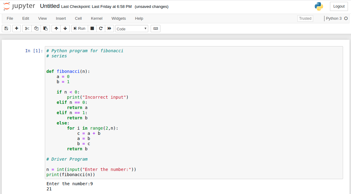
Markdown

Markdown is a popular markup language that is the superset of the HTML. Jupyter Notebook also supports markdown. The cell type can be changed to markdown using the cell menu.  Adding Headers: Heading can be added by prefixing any line by single or multiple ‘#’ followed by space. Example:  Output:  Adding List: Adding List is really simple in Jupyter Notebook. The list can be added by using ‘*’ sign. And the Nested list can be created by using indentation. Example:  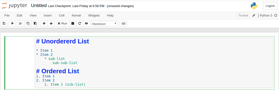Output:  Adding Latex Equations: Latex expressions can be added by surrounding the latex code by ‘$’ and for writing the expressions in the middle, surrounds the latex code by ‘$$’. Example:  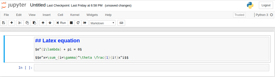Output:  Adding Table: A table can be added by writing the content in the following format.  Output:  Note: The text can be made bold or italic by enclosing the text in ‘**’ and ‘*’ respectively.

Raw NBConverter

Raw cells are provided to write the output directly. This cell is not evaluated by Jupyter notebook. After passing through nbconvert the raw cells arrives in the destination folder without any modification. For example, one can write full Python into a raw cell that can only be rendered by Python only after conversion by nbconvert.

Kernel

A kernel runs behind every notebook. Whenever a cell is executed, the code inside the cell is executed within the kernel and the output is returned back to the cell to be displayed. The kernel continues to exist to the document as a whole and not for individual cells. For example, if a module is imported in one cell then, that module will be available for the whole document. See the below example for better understanding. Example: 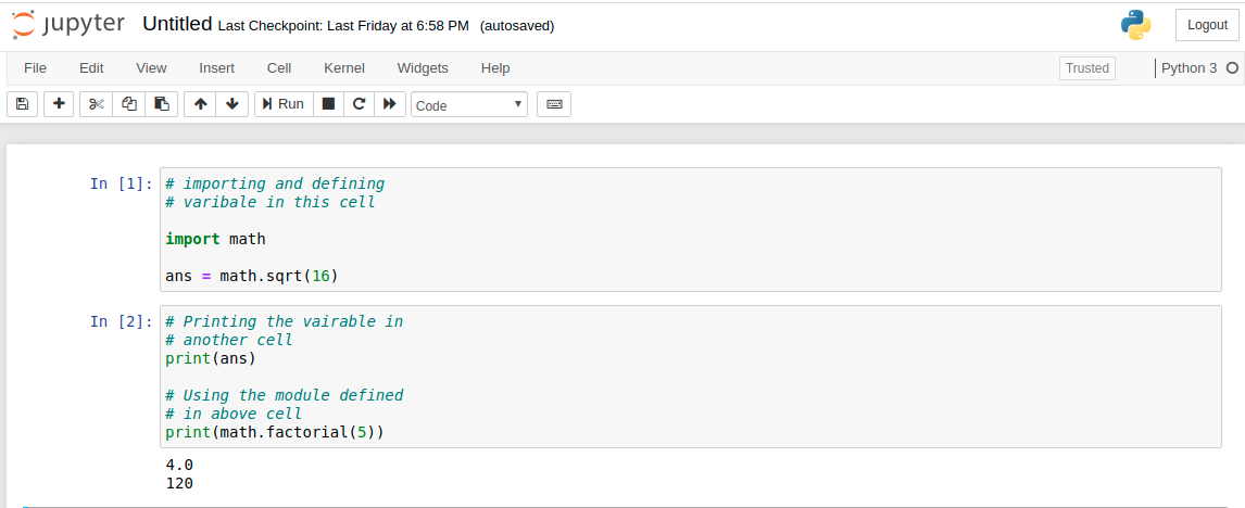 Note: The order of execution of each cell is stated to the left of the cell. In the above example, the cell with In[1] is executed first then the cell with In[2] is executed. Options for kernels: Jupyter Notebook provides various options for kernels. This can be useful if you want to reset things. The options are:

• Restart: This will restart the kernels i.e. clearing all the variables that were defined, clearing the modules that were imported, etc.
• Restart and Clear Output: This will do the same as above but will also clear all the output that was displayed below the cell.
• Restart and Run All: This is also the same as above but will also run all the cells in the top-down order.
• Interrupt: This option will interrupt the kernel execution. It can be useful in the case where the programs continue for execution or the kernel is stuck over some computation.

Naming the notebook

When the notebook is created, Jupyter Notebook names the notebook as Untitled as default. However, the notebook can be renamed. To rename the notebook just click on the word Untitled. This will prompt a dialogue box titled Rename Notebook. Enter the valid name for your notebook in the text bar, then click ok. 

Notebook Extensions

New functionality can be added to Jupyter through extensions. Extensions are javascript module. You can even write your own extension that can access the page’s DOM and the Jupyter Javascript API. Jupyter supports four types of extensions.

• Kernel
• IPyhton Kernel
• Notebook
• Notebook server

The Notebook dashboard

The dashboard contains several tabs which are as follows:

• Files: shows all files and notebooks in the current directory
• Running: shows all kernels currently running on your computer
• Clusters: lets you launch kernels for parallel computing

A notebook is an interactive document containing code, text, and other elements. A notebook is saved in a file with the .ipynb extension. This file is a plain text file storing a JSON data structure.

A kernel is a process running an interactive session. When using IPython, this kernel is a Python process. There are kernels in many languages other than Python.

[box type=”note” align=”alignleft” class=”” width=””]We follow the convention to use the term notebook for a file, and Notebook for the application and the web interface.[/box]

In Jupyter, notebooks and kernels are strongly separated. A notebook is a file, whereas a kernel is a process. The kernel receives snippets of code from the Notebook interface, executes them, and sends the outputs and possible errors back to the Notebook interface. Thus, in general, the kernel has no notion of the Notebook. A notebook is persistent (it’s a file), whereas a kernel may be closed at the end of an interactive session and it is therefore not persistent. When a notebook is re-opened, it needs to be re-executed.

In general, no more than one Notebook interface can be connected to a given kernel. However, several IPython consoles can be connected to a given kernel.

The Notebook user interface

To create a new notebook, click on the New button, and select Notebook (Python 3). A new browser tab opens and shows the Notebook interface as follows:

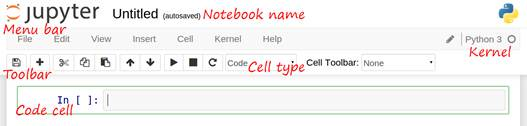
A new notebook

Here are the main components of the interface, from top to bottom:

• The notebook name, which you can change by clicking on it. This is also the name of the .ipynb file.
• The Menu bar gives you access to several actions pertaining to either the notebook or the kernel.
• To the right of the menu bar is the Kernel name. You can change the kernel language of your notebook from the Kernel menu.
• The Toolbar contains icons for common actions. In particular, the dropdown menu showing Code lets you change the type of a cell.
• Following is the main component of the UI: the actual Notebook. It consists of a linear list of cells. We will detail the structure of a cell in the following sections.

Structure of a notebook cell

There are two main types of cells: Markdown cells and code cells, and they are described as follows:

• A Markdown cell contains rich text. In addition to classic formatting options like bold or italics, we can add links, images, HTML elements, LaTeX mathematical equations, and more.
• A code cell contains code to be executed by the kernel. The programming language corresponds to the kernel’s language. We will only use Python in this book, but you can use many other languages.

You can change the type of a cell by first clicking on a cell to select it, and then choosing the cell’s type in the toolbar’s dropdown menu showing Markdown or Code.

Markdown cells

Here is a screenshot of a Markdown cell:

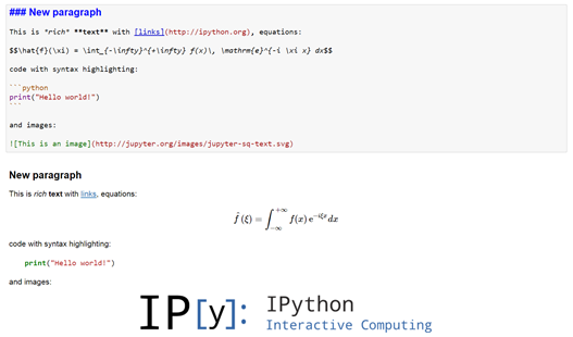
A Markdown cell

The top panel shows the cell in edit mode, while the bottom one shows it in render mode. The edit mode lets you edit the text, while the render mode lets you display the rendered cell. We will explain the differences between these modes in greater detail in the following section.

Code cells

Here is a screenshot of a complex code cell:

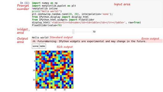
Structure of a code cell

This code cell contains several parts, as follows:

• The Prompt number shows the cell’s number. This number increases every time you run the cell. Since you can run cells of a notebook out of order, nothing guarantees that code numbers are linearly increasing in a given notebook.
• The Input area contains a multiline text editor that lets you write one or several lines of code with syntax highlighting.
• The Widget area may contain graphical controls; here, it displays a slider.
• The Output area can contain multiple outputs, here:
  • Standard output (text in black)
  • Error output (text with a red background)
  • Rich output (an HTML table and an image here)

The Notebook modal interface

The Notebook implements a modal interface similar to some text editors such as vim. Mastering this interface may represent a small learning curve for some users.

• Use the edit mode to write code (the selected cell has a green border, and a pen icon appears at the top right of the interface). Click inside a cell to enable the edit mode for this cell (you need to double-click with Markdown cells).
• Use the command mode to operate on cells (the selected cell has a gray border, and there is no pen icon). Click outside the text area of a cell to enable the command mode (you can also press the Esc key).

Keyboard shortcuts are available in the Notebook interface. Type h to show them. We review here the most common ones (for Windows and Linux; shortcuts for Mac OS X may be slightly different).

Keyboard shortcuts available in both modes

Here are a few keyboard shortcuts that are always available when a cell is selected:

• Ctrl + Enter: run the cell
• Shift + Enter: run the cell and select the cell below
• Alt + Enter: run the cell and insert a new cell below
• Ctrl + S: save the notebook

Keyboard shortcuts available in the edit mode

In the edit mode, you can type code as usual, and you have access to the following keyboard shortcuts:

• Esc: switch to command mode
• Ctrl + Shift + –: split the cell

Keyboard shortcuts available in the command mode

In the command mode, keystrokes are bound to cell operations. Don’t write code in command mode or unexpected things will happen! For example, typing dd in command mode will delete the selected cell! Here are some keyboard shortcuts available in command mode:

• Enter: switch to edit mode
• Up or k: select the previous cell
• Down or j: select the next cell
• y / m: change the cell type to code cell/Markdown cell
• a / b: insert a new cell above/below the current cell
• x / c / v: cut/copy/paste the current cell
• dd: delete the current cell
• z: undo the last delete operation
• Shift + =: merge the cell below
• h: display the help menu with the list of keyboard shortcuts

A crash course on Python

If you don’t know Python, read this section to learn the fundamentals. Python is a very accessible language and is even taught to school children. If you have ever programmed, it will only take you a few minutes to learn the basics.

Hello world

Open a new notebook and type the following in the first cell:

In [1]: print("Hello world!")
Out[1]: Hello world!

Here is a screenshot:

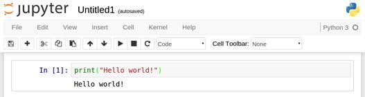
“Hello world” in the Notebook

[box type=”note” align=”alignleft” class=”” width=””]Prompt string

Note that the convention chosen in this article is to show Python code (also called the input) prefixed with In [x]: (which shouldn’t be typed). This is the standard IPython prompt. Here, you should just type print(“Hello world!”) and then press Shift + Enter.[/box]

Congratulations! You are now a Python programmer.

Variables

Let’s use Python as a calculator.

In [2]: 2 * 2
Out[2]: 4

Here, 2 * 2 is an expression statement. This operation is performed, the result is returned, and IPython displays it in the notebook cell’s output.

[box type=”note” align=”alignleft” class=”” width=””]Division

In Python 3, 3 / 2 returns 1.5 (floating-point division), whereas it returns 1 in Python 2 (integer division). This can be source of errors when porting Python 2 code to Python 3. It is recommended to always use the explicit 3.0 / 2.0 for floating-point division (by using floating-point numbers) and 3 // 2 for integer division. Both syntaxes work in Python 2 and Python 3. See http://python3porting.com/differences.html#integer-division for more details.[/box]

Other built-in mathematical operators include +, –, ** for the exponentiation, and others. You will find more details at https://docs.python.org/3/reference/expressions.html#the-power-operator.

Variables form a fundamental concept of any programming language. A variable has a name and a value. Here is how to create a new variable in Python:

In [3]: a = 2

And here is how to use an existing variable:

In [4]: a * 3
Out[4]: 6

Several variables can be defined at once (this is called unpacking):

In [5]: a, b = 2, 6

There are different types of variables. Here, we have used a number (more precisely, an integer). Other important types include floating-point numbers to represent real numbers, strings to represent text, and booleans to represent True/False values. Here are a few examples:

In [6]: somefloat = 3.1415
        sometext = 'pi is about'  # You can also use double quotes.
        print(sometext, somefloat)  # Display several variables.
Out[6]: pi is about 3.1415

Note how we used the # character to write comments. Whereas Python discards the comments completely, adding comments in the code is important when the code is to be read by other humans (including yourself in the future).

String escaping

String escaping refers to the ability to insert special characters in a string. For example, how can you insert ‘ and “, given that these characters are used to delimit a string in Python code? The backslash is the go-to escape character in Python (and in many other languages too). Here are a few examples:

In [7]: print("Hello "world"")
        print("A list:n* item 1n* item 2")
        print("C:pathonwindows")
        print(r"C:pathonwindows")
Out[7]: Hello "world"
        A list:
        * item 1
        * item 2
        C:pathonwindows
        C:pathonwindows

The special character n is the new line (or line feed) character. To insert a backslash, you need to escape it, which explains why it needs to be doubled as .

You can also disable escaping by using raw literals with a r prefix before the string, like in the last example above. In this case, backslashes are considered as normal characters.

This is convenient when writing Windows paths, since Windows uses backslash separators instead of forward slashes like on Unix systems. A very common error on Windows is forgetting to escape backslashes in paths: writing “C:path” may lead to subtle errors.

You will find the list of special characters in Python at

Lists

A list contains a sequence of items. You can concisely instruct Python to perform repeated actions on the elements of a list. Let’s first create a list of numbers as follows:

In [8]: items = [1, 3, 0, 4, 1]

Note the syntax we used to create the list: square brackets [], and commas , to separate the items.

The built-in function len() returns the number of elements in a list:

In [9]: len(items)
Out[9]: 5

[box type=”note” align=”alignleft” class=”” width=””]Python comes with a set of built-in functions, including print(), len(), max(), functional routines like filter() and map(), and container-related routines like all(), any(), range(), and sorted(). You will find the full list of built-in functions at https://docs.python.org/3.4/library/functions.html.[/box]

Now, let’s compute the sum of all elements in the list. Python provides a built-in function for this:

In [10]: sum(items)
Out[10]: 9

We can also access individual elements in the list, using the following syntax:

In [11]: items[0]
Out[11]: 1
In [12]: items[-1]
Out[12]: 1

Note that indexing starts at 0 in Python: the first element of the list is indexed by 0, the second by 1, and so on. Also, -1 refers to the last element, -2, to the penultimate element, and so on.

The same syntax can be used to alter elements in the list:

In [13]: items[1] = 9
         items
Out[13]: [1, 9, 0, 4, 1]

We can access sublists with the following syntax:

In [14]: items[1:3]
Out[14]: [9, 0]

Here, 1:3 represents a slice going from element 1 included (this is the second element of the list) to element 3 excluded. Thus, we get a sublist with the second and third element of the original list. The first-included/last-excluded asymmetry leads to an intuitive treatment of overlaps between consecutive slices. Also, note that a sublist refers to a dynamic view of the original list, not a copy; changing elements in the sublist automatically changes them in the original list.

Python provides several other types of containers:

• Tuples are immutable and contain a fixed number of elements:

  In [15]: my_tuple = (1, 2, 3)
           my_tuple[1]
  Out[15]: 2

• Dictionaries contain key-value pairs. They are extremely useful and common:

  In [16]: my_dict = {'a': 1, 'b': 2, 'c': 3}
           print('a:', my_dict['a'])
  Out[16]: a: 1
  In [17]: print(my_dict.keys())
  Out[17]: dict_keys(['c', 'a', 'b'])
  

  There is no notion of order in a dictionary. However, the native collections module provides an OrderedDict structure that keeps the insertion order (see https://docs.python.org/3.4/library/collections.html).

• Sets, like mathematical sets, contain distinct elements:

  In [18]: my_set = set([1, 2, 3, 2, 1])
           my_set
  Out[18]: {1, 2, 3}
  

A Python object is mutable if its value can change after it has been created. Otherwise, it is immutable. For example, a string is immutable; to change it, a new string needs to be created. A list, a dictionary, or a set is mutable; elements can be added or removed. By contrast, a tuple is immutable, and it is not possible to change the elements it contains without recreating the tuple. See https://docs.python.org/3.4/reference/datamodel.html for more details.

Loops

We can run through all elements of a list using a for loop:

In [19]: for item in items:
             print(item)
Out[19]: 1
         9
         0
         4
         1

There are several things to note here:

• The for item in items syntax means that a temporary variable named item is created at every iteration. This variable contains the value of every item in the list, one at a time.
• Note the colon : at the end of the for statement. Forgetting it will lead to a syntax error!
• The statement print(item) will be executed for all items in the list.
• Note the four spaces before print: this is called the indentation. You will find more details about indentation in the next subsection.

Python supports a concise syntax to perform a given operation on all elements of a list, as follows:

In [20]: squares = [item * item for item in items]
         squares
Out[20]: [1, 81, 0, 16, 1]

This is called a list comprehension. A new list is created here; it contains the squares of all numbers in the list. This concise syntax leads to highly readable and Pythonic code.

Indentation

Indentation refers to the spaces that may appear at the beginning of some lines of code. This is a particular aspect of Python’s syntax.

In most programming languages, indentation is optional and is generally used to make the code visually clearer. But in Python, indentation also has a syntactic meaning. Particular indentation rules need to be followed for Python code to be correct.

In general, there are two ways to indent some text: by inserting a tab character (also referred to as t), or by inserting a number of spaces (typically, four). It is recommended to use spaces instead of tab characters. Your text editor should be configured such that the Tab key on the keyboard inserts four spaces instead of a tab character.

In the Notebook, indentation is automatically configured properly; so you shouldn’t worry about this issue. The question only arises if you use another text editor for your Python code.

Finally, what is the meaning of indentation? In Python, indentation delimits coherent blocks of code, for example, the contents of a loop, a conditional branch, a function, and other objects. Where other languages such as C or JavaScript use curly braces to delimit such blocks, Python uses indentation.

Conditional branches

Sometimes, you need to perform different operations on your data depending on some condition. For example, let’s display all even numbers in our list:

In [21]: for item in items:
             if item % 2 == 0:
                 print(item)
Out[21]: 0
         4

Again, here are several things to note:

• An if statement is followed by a boolean expression.
• If a and b are two integers, the modulo operand a % b returns the remainder from the division of a by b. Here, item % 2 is 0 for even numbers, and 1 for odd numbers.
• The equality is represented by a double equal sign == to avoid confusion with the assignment operator = that we use when we create variables.
• Like with the for loop, the if statement ends with a colon :.
• The part of the code that is executed when the condition is satisfied follows the if statement. It is indented. Indentation is cumulative: since this if is inside a for loop, there are eight spaces before the print(item) statement.

Python supports a concise syntax to select all elements in a list that satisfy certain properties. Here is how to create a sublist with only even numbers:

In [22]: even = [item for item in items if item % 2 == 0]
         even
Out[22]: [0, 4]

This is also a form of list comprehension.

Functions

Code is typically organized into functions. A function encapsulates part of your code. Functions allow you to reuse bits of functionality without copy-pasting the code. Here is a function that tells whether an integer number is even or not:

In [23]: def is_even(number):
             """Return whether an integer is even or not."""
             return number % 2 == 0

There are several things to note here:

• A function is defined with the def keyword.
• After def comes the function name. A general convention in Python is to only use lowercase characters, and separate words with an underscore _. A function name generally starts with a verb.
• The function name is followed by parentheses, with one or several variable names called the arguments. These are the inputs of the function. There is a single argument here, named number.
• No type is specified for the argument. This is because Python is dynamically typed; you could pass a variable of any type. This function would work fine with floating point numbers, for example (the modulo operation works with floating point numbers in addition to integers).
• The body of the function is indented (and note the colon : at the end of the def statement).
• There is a docstring wrapped by triple quotes “””. This is a particular form of comment that explains what the function does. It is not mandatory, but it is strongly recommended to write docstrings for the functions exposed to the user.
• The return keyword in the body of the function specifies the output of the function. Here, the output is a Boolean, obtained from the expression number % 2 == 0. It is possible to return several values; just use a comma to separate them (in this case, a tuple of Booleans would be returned).

Once a function is defined, it can be called like this:

In [24]: is_even(3)
Out[24]: False
In [25]: is_even(4)
Out[25]: True

Here, 3 and 4 are successively passed as arguments to the function.

Positional and keyword arguments

A Python function can accept an arbitrary number of arguments, called positional arguments. It can also accept optional named arguments, called keyword arguments. Here is an example:

In [26]: def remainder(number, divisor=2):
             return number % divisor

The second argument of this function, divisor, is optional. If it is not provided by the caller, it will default to the number 2, as shown here:

In [27]: remainder(5)
Out[27]: 1

There are two equivalent ways of specifying a keyword argument when calling a function. They are as follows:

In [28]: remainder(5, 3)
Out[28]: 2
In [29]: remainder(5, divisor=3)
Out[29]: 2

In the first case, 3 is understood as the second argument, divisor. In the second case, the name of the argument is given explicitly by the caller. This second syntax is clearer and less error-prone than the first one.

Functions can also accept arbitrary sets of positional and keyword arguments, using the following syntax:

In [30]: def f(*args, **kwargs):
             print("Positional arguments:", args)
             print("Keyword arguments:", kwargs)
In [31]: f(1, 2, c=3, d=4)
Out[31]: Positional arguments: (1, 2)
         Keyword arguments: {'c': 3, 'd': 4}

Inside the function, args is a tuple containing positional arguments, and kwargs is a dictionary containing keyword arguments.

Passage by assignment

When passing a parameter to a Python function, a reference to the object is actually passed (passage by assignment):

• If the passed object is mutable, it can be modified by the function
• If the passed object is immutable, it cannot be modified by the function

Here is an example:

In [32]: my_list = [1, 2]

         def add(some_list, value):
             some_list.append(value)

         add(my_list, 3)
         my_list
Out[32]: [1, 2, 3]

The add() function modifies an object defined outside it (in this case, the object my_list); we say this function has side-effects. A function with no side-effects is called a pure function: it doesn’t modify anything in the outer context, and it deterministically returns the same result for any given set of inputs. Pure functions are to be preferred over functions with side-effects.

Knowing this can help you spot out subtle bugs. There are further related concepts that are useful to know, including function scopes, naming, binding, and more. Here are a couple of links:

• Passage by reference at https://docs.python.org/3/faq/programming.html#how-do-i-write-a-function-with-output-parameters-call-by-reference
• Naming, binding, and scope at https://docs.python.org/3.4/reference/executionmodel.html

Errors

Let’s discuss errors in Python. As you learn, you will inevitably come across errors and exceptions. The Python interpreter will most of the time tell you what the problem is, and where it occurred. It is important to understand the vocabulary used by Python so that you can more quickly find and correct your errors.

Let’s see the following example:

In [33]: def divide(a, b):
             return a / b
In [34]: divide(1, 0)
Out[34]: ---------------------------------------------------------
         ZeroDivisionError       Traceback (most recent call last)
         <ipython-input-2-b77ebb6ac6f6> in <module>()
         ----> 1 divide(1, 0)

         <ipython-input-1-5c74f9fd7706> in divide(a, b)
               1 def divide(a, b):
         ----> 2     return a / b

         ZeroDivisionError: division by zero

Here, we defined a divide() function, and called it to divide 1 by 0. Dividing a number by 0 is an error in Python. Here, a ZeroDivisionError exception was raised. An exception is a particular type of error that can be raised at any point in a program. It is propagated from the innards of the code up to the command that launched the code. It can be caught and processed at any point. You will find more details about exceptions at https://docs.python.org/3/tutorial/errors.html, and common exception types at https://docs.python.org/3/library/exceptions.html#bltin-exceptions.

The error message you see contains the stack trace, the exception type, and the exception message. The stack trace shows all function calls between the raised exception and the script calling point.

The top frame, indicated by the first arrow —->, shows the entry point of the code execution. Here, it is divide(1, 0), which was called directly in the Notebook. The error occurred while this function was called.

The next and last frame is indicated by the second arrow. It corresponds to line 2 in our function divide(a, b). It is the last frame in the stack trace: this means that the error occurred there.

Object-oriented programming

Object-oriented programming (OOP) is a relatively advanced topic. Although we won’t use it much in this book, it is useful to know the basics. Also, mastering OOP is often essential when you start to have a large code base.

In Python, everything is an object. A number, a string, or a function is an object. An object is an instance of a type (also known as class). An object has attributes and methods, as specified by its type. An attribute is a variable bound to an object, giving some information about it. A method is a function that applies to the object.

For example, the object ‘hello’ is an instance of the built-in str type (string). The type() function returns the type of an object, as shown here:

In [35]: type('hello')
Out[35]: str

There are native types, like str or int (integer), and custom types, also called classes, that can be created by the user.

In IPython, you can discover the attributes and methods of any object with the dot syntax and tab completion. For example, typing ‘hello’.u and pressing Tab automatically shows us the existence of the upper() method:

In [36]: 'hello'.upper()
Out[36]: 'HELLO'

Here, upper() is a method available to all str objects; it returns an uppercase copy of a string.

A useful string method is format(). This simple and convenient templating system lets you generate strings dynamically, as shown in the following example:

In [37]: 'Hello {0:s}!'.format('Python')
Out[37]: Hello Python

The {0:s} syntax means “replace this with the first argument of format(), which should be a string”. The variable type after the colon is especially useful for numbers, where you can specify how to display the number (for example, .3f to display three decimals). The 0 makes it possible to replace a given value several times in a given string. You can also use a name instead of a position—for example ‘Hello {name}!’.format(name=’Python’).

Some methods are prefixed with an underscore _; they are private and are generally not meant to be used directly. IPython’s tab completion won’t show you these private attributes and methods unless you explicitly type _ before pressing Tab.

In practice, the most important thing to remember is that appending a dot . to any Python object and pressing Tab in IPython will show you a lot of functionality pertaining to that object.

Functional programming

Python is a multi-paradigm language; it notably supports imperative, object-oriented, and functional programming models. Python functions are objects and can be handled like other objects. In particular, they can be passed as arguments to other functions (also called higher-order functions). This is the essence of functional programming.

Decorators provide a convenient syntax construct to define higher-order functions. Here is an example using the is_even() function from the previous Functions section:

In [38]: def show_output(func):
             def wrapped(*args, **kwargs):
                 output = func(*args, **kwargs)
                 print("The result is:", output)
             return wrapped

The show_output() function transforms an arbitrary function func() to a new function, named wrapped(), that displays the result of the function, as follows:

In [39]: f = show_output(is_even)
         f(3)
Out[39]: The result is: False

Equivalently, this higher-order function can also be used with a decorator, as follows:

In [40]: @show_output
         def square(x):
             return x * x
In [41]: square(3)
Out[41]: The result is: 9